02. Post-stack inversion

This tutorial focuses on extending post-stack seismic inversion to GPU processing. We refer to the equivalent PyLops tutorial for a more detailed description of the theory.

# sphinx_gallery_thumbnail_number = 2
import numpy as np
import torch
import matplotlib.pyplot as plt
from scipy.signal import filtfilt
from pylops.utils.wavelets import ricker

import pylops_gpu
from pylops_gpu.utils.backend import device

dev = device()
plt.close('all')
np.random.seed(10)
torch.manual_seed(10)

Out:

<torch._C.Generator object at 0x7fbc865527b0>

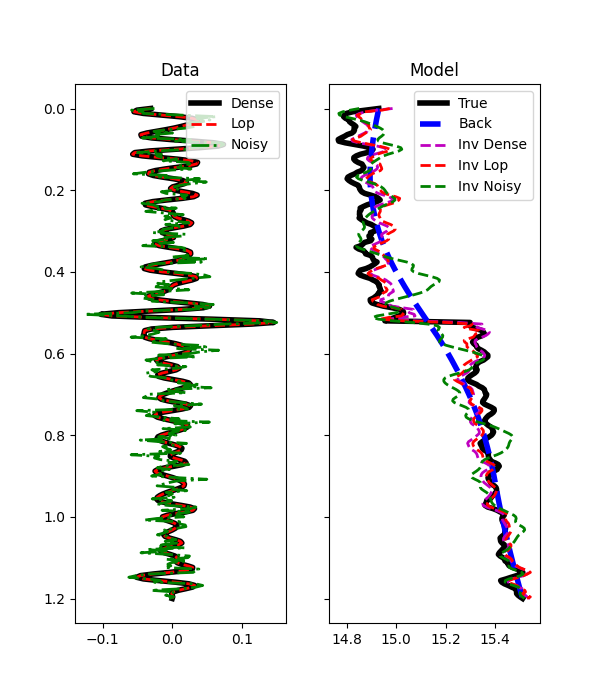
We consider the 1d example. A synthetic profile of acoustic impedance is created and data is modelled using both the dense and linear operator version of pylops_gpu.avo.poststack.PoststackLinearModelling operator. Both model and wavelet are created as numpy arrays and converted into torch tensors (note that we enforce float32 for optimal performance on GPU).

# model
nt0 = 301
dt0 = 0.004
t0 = np.arange(nt0)*dt0
vp = 1200 + np.arange(nt0) + \
     filtfilt(np.ones(5)/5., 1, np.random.normal(0, 80, nt0))
rho = 1000 + vp + \
      filtfilt(np.ones(5)/5., 1, np.random.normal(0, 30, nt0))
vp[131:] += 500
rho[131:] += 100
m = np.log(vp*rho)

# smooth model
nsmooth = 100
mback = filtfilt(np.ones(nsmooth)/float(nsmooth), 1, m)

# wavelet
ntwav = 41
wav, twav, wavc = ricker(t0[:ntwav//2+1], 20)

# convert to torch tensors
m = torch.from_numpy(m.astype('float32'))
mback = torch.from_numpy(mback.astype('float32'))
wav = torch.from_numpy(wav.astype('float32'))

# dense operator
PPop_dense = \
    pylops_gpu.avo.poststack.PoststackLinearModelling(wav / 2, nt0=nt0,
                                                      explicit=True)

# lop operator
PPop = pylops_gpu.avo.poststack.PoststackLinearModelling(wav / 2, nt0=nt0)

# data
d_dense = PPop_dense * m.flatten()
d = PPop * m.flatten()

# add noise
dn_dense = d_dense + \
           torch.from_numpy(np.random.normal(0, 2e-2, d_dense.shape).astype('float32'))

We can now estimate the acoustic profile from band-limited data using either the dense operator or linear operator.

# solve dense
minv_dense = \
    pylops_gpu.avo.poststack.PoststackInversion(d, wav / 2, m0=mback, explicit=True,
                                                simultaneous=False)[0]

# solve lop
minv = \
    pylops_gpu.avo.poststack.PoststackInversion(d_dense, wav / 2, m0=mback,
                                                explicit=False,
                                                simultaneous=False,
                                                **dict(niter=500))[0]

# solve noisy
mn = \
    pylops_gpu.avo.poststack.PoststackInversion(dn_dense, wav / 2, m0=mback,
                                                explicit=True, epsI=1e-4,
                                                epsR=1e0, **dict(niter=100))[0]


fig, axs = plt.subplots(1, 2, figsize=(6, 7), sharey=True)
axs[0].plot(d_dense, t0, 'k', lw=4, label='Dense')
axs[0].plot(d, t0, '--r', lw=2, label='Lop')
axs[0].plot(dn_dense, t0, '-.g', lw=2, label='Noisy')
axs[0].set_title('Data')
axs[0].invert_yaxis()
axs[0].axis('tight')
axs[0].legend(loc=1)
axs[1].plot(m, t0, 'k', lw=4, label='True')
axs[1].plot(mback, t0, '--b', lw=4, label='Back')
axs[1].plot(minv_dense, t0, '--m', lw=2, label='Inv Dense')
axs[1].plot(minv, t0, '--r', lw=2, label='Inv Lop')
axs[1].plot(mn, t0, '--g', lw=2, label='Inv Noisy')
axs[1].set_title('Model')
axs[1].axis('tight')
axs[1].legend(loc=1)

Out:

<matplotlib.legend.Legend object at 0x7fbc634cb3c8>

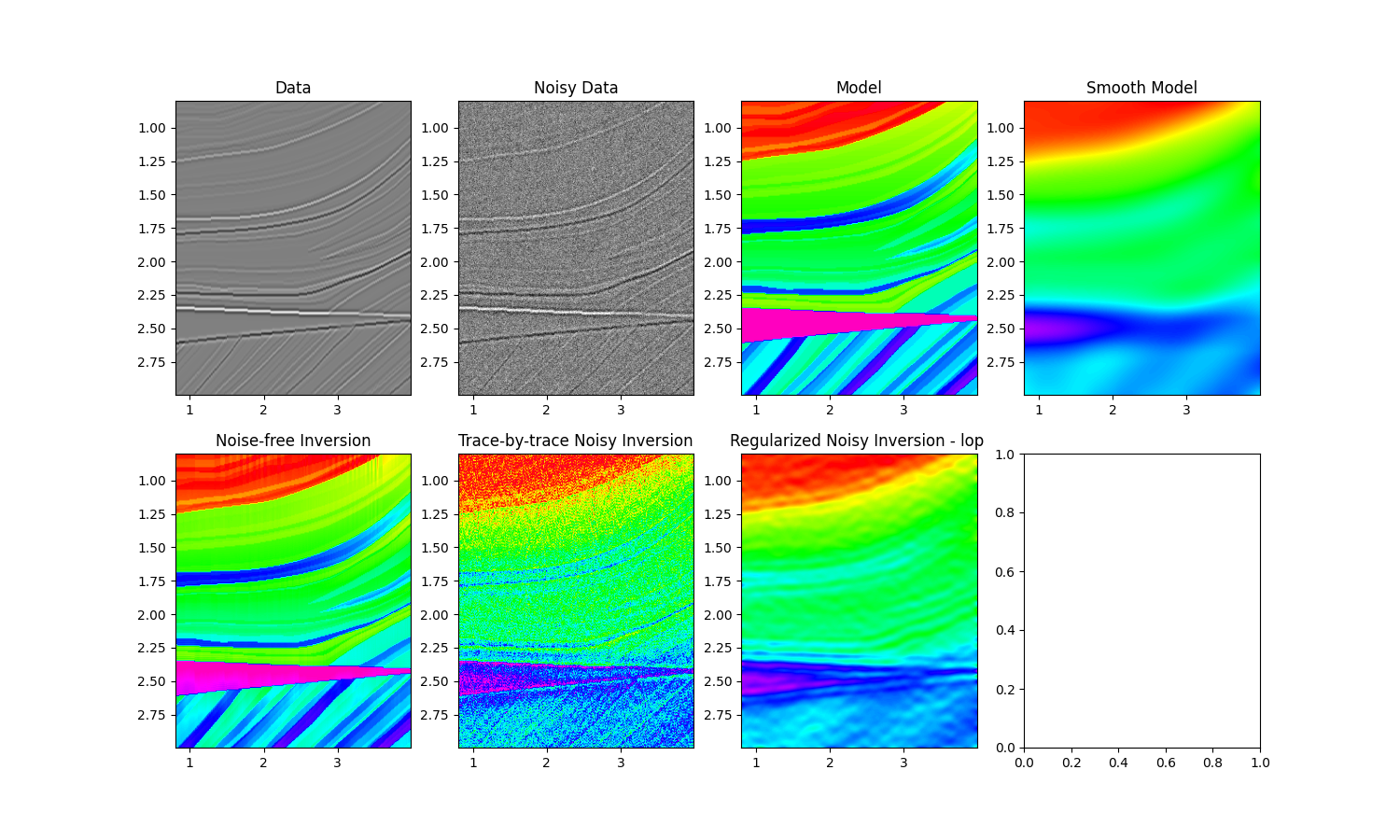
We move now to a 2d example. First of all the model is loaded and data generated.

# model
inputfile = '../testdata/avo/poststack_model.npz'

model = np.load(inputfile)
m = np.log(model['model'][:, ::3])
x, z = model['x'][::3]/1000., model['z']/1000.
nx, nz = len(x), len(z)


# smooth model
nsmoothz, nsmoothx = 60, 50
mback = filtfilt(np.ones(nsmoothz)/float(nsmoothz), 1, m, axis=0)
mback = filtfilt(np.ones(nsmoothx)/float(nsmoothx), 1, mback, axis=1)

# convert to torch tensors
m = torch.from_numpy(m.astype('float32'))
mback = torch.from_numpy(mback.astype('float32'))


# dense operator
PPop_dense = \
    pylops_gpu.avo.poststack.PoststackLinearModelling(wav / 2, nt0=nz,
                                                      spatdims=nx, explicit=True)

# lop operator
PPop = pylops_gpu.avo.poststack.PoststackLinearModelling(wav / 2, nt0=nz,
                                                         spatdims=nx)

# data
d = (PPop_dense * m.flatten()).reshape(nz, nx)
n = torch.from_numpy(np.random.normal(0, 1e-1, d.shape).astype('float32'))
dn = d + n

Finally we perform different types of inversion

# dense inversion with noise-free data
minv_dense = \
    pylops_gpu.avo.poststack.PoststackInversion(d, wav / 2, m0=mback,
                                                explicit=True,
                                                simultaneous=False)[0]

# dense inversion with noisy data
minv_dense_noisy = \
    pylops_gpu.avo.poststack.PoststackInversion(dn, wav / 2, m0=mback,
                                                explicit=True, epsI=4e-2,
                                                simultaneous=False)[0]

# spatially regularized lop inversion with noisy data
minv_lop_reg = \
    pylops_gpu.avo.poststack.PoststackInversion(dn, wav / 2, m0=minv_dense_noisy,
                                                explicit=False,
                                                epsR=5e1, epsI=1e-2,
                                                **dict(niter=80))[0]

fig, axs = plt.subplots(2, 4, figsize=(15, 9))
axs[0][0].imshow(d, cmap='gray',
                 extent=(x[0], x[-1], z[-1], z[0]),
                 vmin=-0.4, vmax=0.4)
axs[0][0].set_title('Data')
axs[0][0].axis('tight')
axs[0][1].imshow(dn, cmap='gray',
                 extent=(x[0], x[-1], z[-1], z[0]),
                 vmin=-0.4, vmax=0.4)
axs[0][1].set_title('Noisy Data')
axs[0][1].axis('tight')
axs[0][2].imshow(m, cmap='gist_rainbow',
                 extent=(x[0], x[-1], z[-1], z[0]),
                 vmin=m.min(), vmax=m.max())
axs[0][2].set_title('Model')
axs[0][2].axis('tight')
axs[0][3].imshow(mback, cmap='gist_rainbow',
                 extent=(x[0], x[-1], z[-1], z[0]),
                 vmin=m.min(), vmax=m.max())
axs[0][3].set_title('Smooth Model')
axs[0][3].axis('tight')
axs[1][0].imshow(minv_dense, cmap='gist_rainbow',
                 extent=(x[0], x[-1], z[-1], z[0]),
                 vmin=m.min(), vmax=m.max())
axs[1][0].set_title('Noise-free Inversion')
axs[1][0].axis('tight')
axs[1][1].imshow(minv_dense_noisy, cmap='gist_rainbow',
                 extent=(x[0], x[-1], z[-1], z[0]),
                 vmin=m.min(), vmax=m.max())
axs[1][1].set_title('Trace-by-trace Noisy Inversion')
axs[1][1].axis('tight')
axs[1][2].imshow(minv_lop_reg, cmap='gist_rainbow',
                 extent=(x[0], x[-1], z[-1], z[0]),
                 vmin=m.min(), vmax=m.max())
axs[1][2].set_title('Regularized Noisy Inversion - lop ')
axs[1][2].axis('tight')

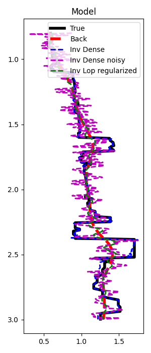
fig, ax = plt.subplots(1, 1, figsize=(3, 7))
ax.plot(m[:, nx//2], z, 'k', lw=4, label='True')
ax.plot(mback[:, nx//2], z, '--r', lw=4, label='Back')
ax.plot(minv_dense[:, nx//2], z, '--b', lw=2, label='Inv Dense')
ax.plot(minv_dense_noisy[:, nx//2], z, '--m', lw=2, label='Inv Dense noisy')
ax.plot(minv_lop_reg[:, nx//2], z, '--g', lw=2, label='Inv Lop regularized')
ax.set_title('Model')
ax.invert_yaxis()
ax.axis('tight')
ax.legend()
plt.tight_layout()

• 
• 

Finally, if you want to run this code on GPUs, take a look at the following notebook and obtain more and more speed-up for problems of increasing size.