Total Variation (TV) Regularization

This set of examples shows how to add Total Variation (TV) regularization to an inverse problem in order to enforce blockiness in the reconstructed model.

To do so we will use the generalizated Split Bregman iterations by means of pylops_gpu.optimization.sparsity.SplitBregman solver.

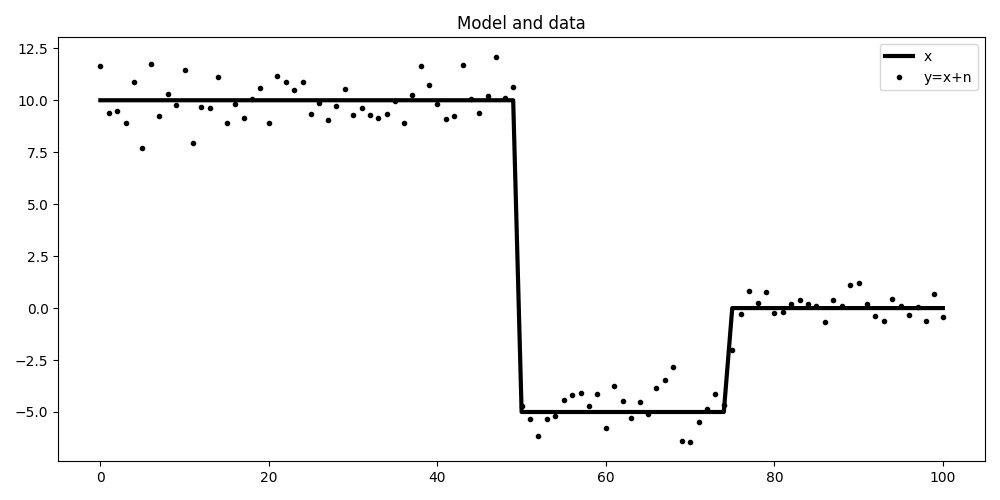
The first example is concerned with denoising of a piece-wise step function which has been contaminated by noise. The forward model is:

\[\mathbf{y} = \mathbf{x} + \mathbf{n}\]

meaning that we have an identity operator (\(\mathbf{I}\)) and inverting for \(\mathbf{x}\) from \(\mathbf{y}\) is impossible without adding prior information. We will enforce blockiness in the solution by adding a regularization term that enforces sparsity in the first derivative of the solution:

\[J = \mu/2 ||\mathbf{y} - \mathbf{I} \mathbf{x}||_2 + || \nabla \mathbf{x}||_1\]

# sphinx_gallery_thumbnail_number = 3
import torch
import numpy as np
import matplotlib.pyplot as plt
import pylops_gpu

from pylops_gpu.utils.backend import device

dev = device()
print('PyLops-gpu working on %s...' % dev)
plt.close('all')

torch.manual_seed(0)
np.random.seed(1)
dtype = torch.float32

Out:

PyLops-gpu working on cpu...

Let’s start by creating the model and data

nx = int(101)
x = torch.zeros(nx, dtype=dtype).to(dev)
x[:nx//2] = 10
x[nx//2:3*nx//4] = -5
Iop = pylops_gpu.Identity(nx, device=dev, dtype=dtype)
noise = torch.from_numpy(np.random.normal(0, 1, nx).astype(np.float32)).to(dev)

y = Iop * (x + noise)

plt.figure(figsize=(10, 5))
plt.plot(x.cpu(), 'k', lw=3, label='x')
plt.plot(y.cpu(), '.k', label='y=x+n')
plt.legend()
plt.title('Model and data')
plt.tight_layout()

To start we will try to use a simple L2 regularization that enforces smoothness in the solution. We can see how denoising is succesfully achieved but the solution is much smoother than we wish for.

D2op = pylops_gpu.SecondDerivative(nx, device=dev, dtype=dtype)
lamda = 1e2

xinv = xinv = \
    pylops_gpu.optimization.leastsquares.NormalEquationsInversion(Op=Iop,
                                                                  Regs=[D2op],
                                                                  epsRs=[np.sqrt(lamda/2)],
                                                                  data=y,
                                                                  device=dev,
                                                                  **dict(niter=30))

plt.figure(figsize=(10, 5))
plt.plot(x.cpu(), 'k', lw=3, label='x')
plt.plot(y.cpu(), '.k', label='y=x+n')
plt.plot(xinv.cpu(), 'r', lw=5, label='xinv')
plt.legend()
plt.title('L2 inversion')
plt.tight_layout()

Now we impose blockiness in the solution using the Split Bregman solver

Dop = pylops_gpu.FirstDerivative(nx, device=dev, dtype=dtype)
mu = 0.01
lamda = 0.3
niter_out = 50
niter_in = 3

xinv, niter = \
    pylops_gpu.optimization.sparsity.SplitBregman(Iop, [Dop], y, niter_out,
                                                  niter_in, mu=mu, epsRL1s=[lamda],
                                                  tol=1e-4, tau=1.,
                                                  **dict(niter=30, epsI=1e-10))

plt.figure(figsize=(10, 5))
plt.plot(x.cpu(), 'k', lw=3, label='x')
plt.plot(y.cpu(), '.k', label='y=x+n')
plt.plot(xinv.cpu(), 'r', lw=5, label='xinv')
plt.legend()
plt.title('TV inversion')
plt.tight_layout()