Derivatives

This example shows how to use the suite of derivative operators, namely pylops_gpu.FirstDerivative, pylops_gpu.SecondDerivative and pylops_gpu.Laplacian.

The derivative operators are very useful when the model to be inverted for is expect to be smooth in one or more directions. These operators can in fact be used as part of the regularization term to obtain a smooth solution.

import torch
import numpy as np
import matplotlib.pyplot as plt
import pylops_gpu

from pylops_gpu.utils.backend import device

dev = device()
print('PyLops-gpu working on %s...' % dev)
plt.close('all')

Out:

PyLops-gpu working on cpu...

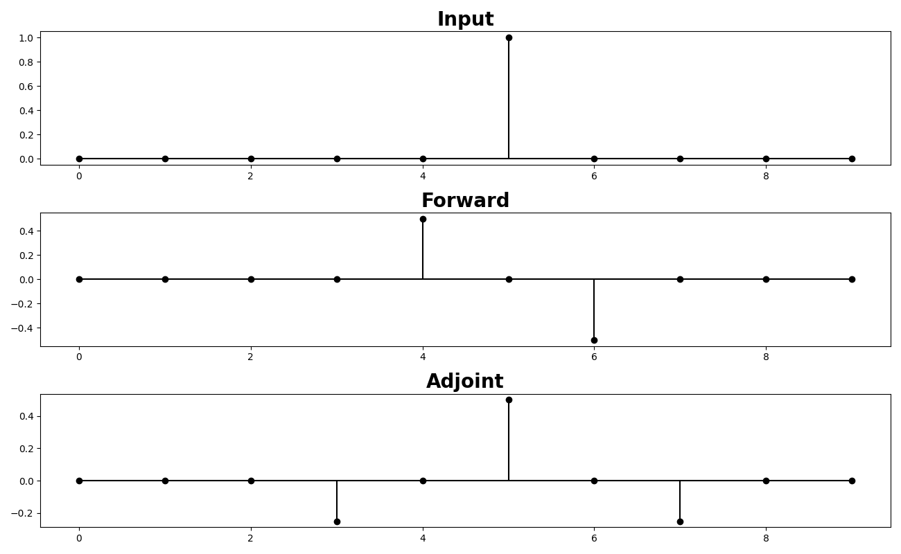
Let’s start by looking at a simple first-order centered derivative. We compute it by means of the pylops_gpu.FirstDerivative operator.

nx = 10
x = torch.zeros(nx, dtype=torch.float32)
x[int(nx/2)] = 1

D1op = pylops_gpu.FirstDerivative(nx, dtype=torch.float32)

y_lop = D1op*x
xadj_lop = D1op.H*y_lop

fig, axs = plt.subplots(3, 1, figsize=(13, 8))
axs[0].stem(np.arange(nx), x, basefmt='k', linefmt='k',
            markerfmt='ko', use_line_collection=True)
axs[0].set_title('Input', size=20, fontweight='bold')
axs[1].stem(np.arange(nx), y_lop, basefmt='k', linefmt='k',
            markerfmt='ko', use_line_collection=True)
axs[1].set_title('Forward', size=20, fontweight='bold')
axs[2].stem(np.arange(nx), xadj_lop, basefmt='k', linefmt='k',
            markerfmt='ko', use_line_collection=True)
axs[2].set_title('Adjoint', size=20, fontweight='bold')
plt.tight_layout()

Let’s move onto applying the same first derivative to a 2d array in the first direction

nx, ny = 11, 21
A = torch.zeros((nx, ny), dtype=torch.float32)
A[nx//2, ny//2] = 1.

D1op = pylops_gpu.FirstDerivative(nx * ny, dims=(nx, ny),
                                  dir=0, dtype=torch.float32)
B = torch.reshape(D1op * A.flatten(), (nx, ny))

fig, axs = plt.subplots(1, 2, figsize=(10, 3))
fig.suptitle('First Derivative in 1st direction', fontsize=12,
             fontweight='bold', y=0.95)
im = axs[0].imshow(A, interpolation='nearest', cmap='rainbow')
axs[0].axis('tight')
axs[0].set_title('x')
plt.colorbar(im, ax=axs[0])
im = axs[1].imshow(B, interpolation='nearest', cmap='rainbow')
axs[1].axis('tight')
axs[1].set_title('y')
plt.colorbar(im, ax=axs[1])
plt.tight_layout()
plt.subplots_adjust(top=0.8)

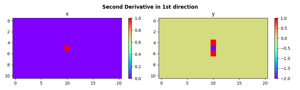
We can now do the same for the second derivative

A = torch.zeros((nx, ny), dtype=torch.float32)
A[nx//2, ny//2] = 1.

D2op = pylops_gpu.SecondDerivative(nx * ny, dims=(nx, ny),
                                   dir=0, dtype=torch.float32)
B = torch.reshape(D2op * A.flatten(), (nx, ny))

fig, axs = plt.subplots(1, 2, figsize=(10, 3))
fig.suptitle('Second Derivative in 1st direction', fontsize=12,
             fontweight='bold', y=0.95)
im = axs[0].imshow(A, interpolation='nearest', cmap='rainbow')
axs[0].axis('tight')
axs[0].set_title('x')
plt.colorbar(im, ax=axs[0])
im = axs[1].imshow(B, interpolation='nearest', cmap='rainbow')
axs[1].axis('tight')
axs[1].set_title('y')
plt.colorbar(im, ax=axs[1])
plt.tight_layout()
plt.subplots_adjust(top=0.8)

And finally we use the symmetrical Laplacian operator as well as a asymmetrical version of it (by adding more weight to the derivative along one direction)

# symmetrical
L2symop = pylops_gpu.Laplacian(dims=(nx, ny), weights=(1, 1),
                               dtype=torch.float32)

# asymmetrical
L2asymop = pylops_gpu.Laplacian(dims=(nx, ny), weights=(3, 1),
                                dtype=torch.float32)

Bsym = torch.reshape(L2symop * A.flatten(), (nx, ny))
Basym = torch.reshape(L2asymop * A.flatten(), (nx, ny))

fig, axs = plt.subplots(1, 3, figsize=(10, 3))
fig.suptitle('Laplacian', fontsize=12,
             fontweight='bold', y=0.95)
im = axs[0].imshow(A, interpolation='nearest', cmap='rainbow')
axs[0].axis('tight')
axs[0].set_title('x')
plt.colorbar(im, ax=axs[0])
im = axs[1].imshow(Bsym, interpolation='nearest', cmap='rainbow')
axs[1].axis('tight')
axs[1].set_title('y sym')
plt.colorbar(im, ax=axs[1])
im = axs[2].imshow(Basym, interpolation='nearest', cmap='rainbow')
axs[2].axis('tight')
axs[2].set_title('y asym')
plt.colorbar(im, ax=axs[2])
plt.tight_layout()
plt.subplots_adjust(top=0.8)